Bixbyite – magnetic

Getting started on analysis.sns.gov

1. Open a terminal (Ctrl+Alt+T)
2. Create a directory on your Desktop mkdir ~/Desktop/Workshop/
3. Copy over CIF and data files cp /SNS/software/scd/examples/bixbyite.* ~/Desktop/Workshop/
4. Launch rmc-discord /SNS/software/scd/rmc-discord.sh

RMC refinement

There are four main steps to performing a reverse Monte Carlo refinement:

1. Define a supercell
2. Load and preprocess a diffuse scattering intensity dataset
3. Setup and perform a refinement
4. Calculate and visualize the correlations

Crystal tab

To define a supercell, it is first necessary to construct a unit cell from the average structure.

1. Begin by loading a crystallographic information file (CIF) or magnetic CIF file
   • The button is located on the upper left corner of window Load CIF.
   • Choose bixbyite.cif.
   • The parameters are extracted from the CIF file and populated into two tables.
   • The left hand table displays all atoms in the unit supercell.
   • The right hand table gives the basic atom site information.
     • Modifying the atom site information on the right automatically updates the unit cell table on the right.
2. Modify (if necessary) the atom site table
   • Begin by choosing between Neutron and X-ray refinement in the upper right combo box.
   • By selecting refinement type first, the relevant parameters are available to edit including nuclei and ions.
     • For magnetic refinement, Neutron must be selected to access magnetic information.
   • To display, different parameters, choose from Site parameters, Structural parameters, and if available Magnetic parameters.
     • In Site parameters, along with the atom (isotope for neutron, ion for X-ray), its occupancy and fractional coordinates \(u\), \(v\), \(w\) can be modified. An atom may also be de-activated or activated for refinement.
     • In Structural parameters, the anisotropic displacement parameters \(U_{ij}\) may be modified. The equivalent isotropic parameter \(U_\text{iso}\) and its principal components will be updated (\(U_1\), \(U_2\), \(U_3\)). If available, Magnetic parameters allows the magnetic ion to be chosen along with the magnetic moment component along the crystal axes. If a valid .mcif is used, the magnetic symmetry will be accounted for. The \(g\)-factor can also be specified.
   • Select Magnetic parameters, choose \(\mathrm{Fe3+}\) and \(\mathrm{Mn3+}\) ions and deactivate site 3 since oxygen is nonmagnetic.
   • Update the occupancy of the Fe-rich site at \((0,0,0)\) to 1.0 and deactivate the Mn-deficient part.
   • Update the occupancy of the Mn site at \((0,0.75,z)\) to 1.0 and deactivate Fe part.
   • Create a supercell with size \(N_1=4\), \(N_2=4\), and \(N_3=4\) by entering the number of cells along each crystal axes.
3. Optionally save the CIF file of the supercell and visualize it in external program VESTA

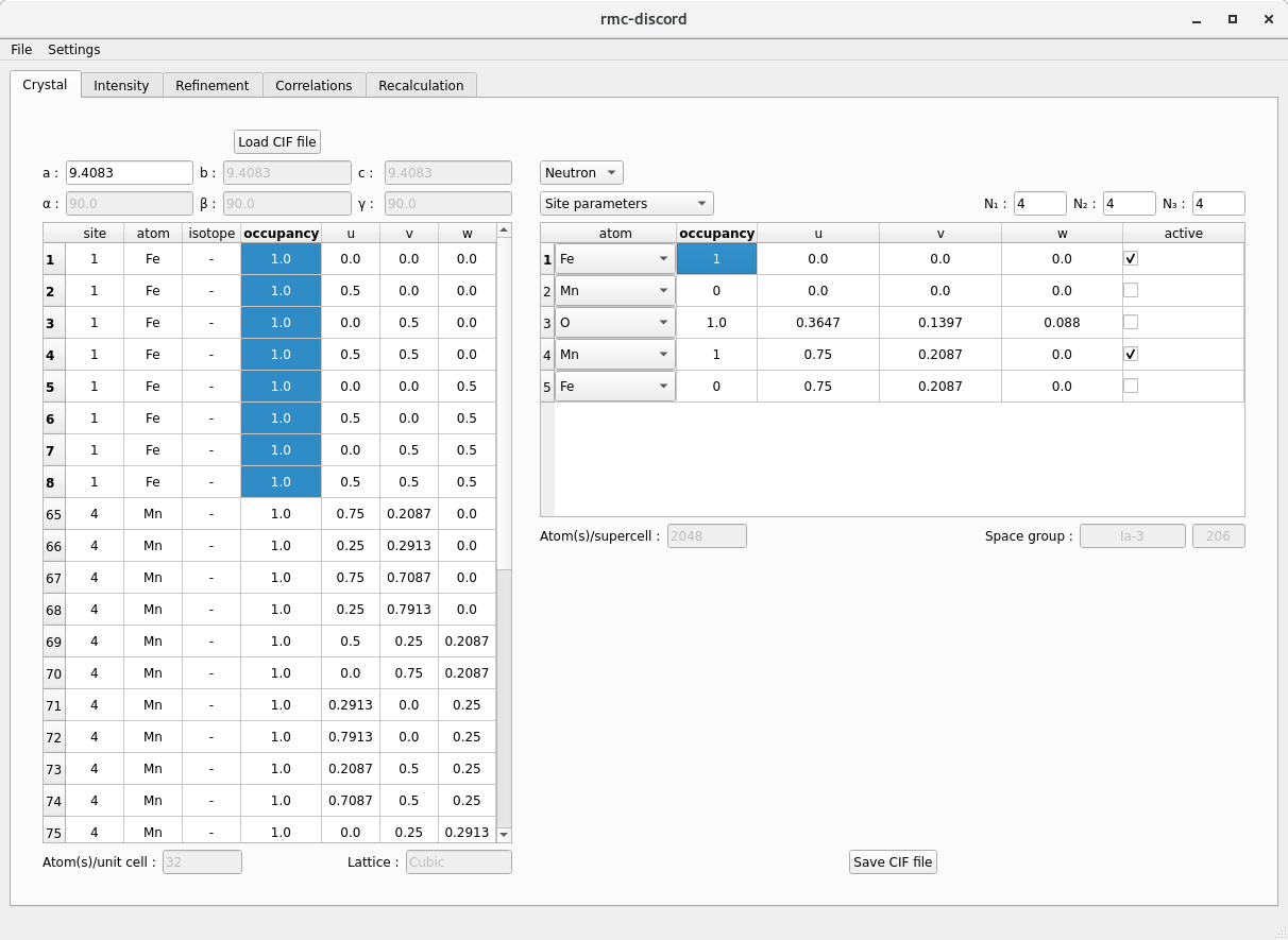
Crystal tab

Hints

• The size of the supercell defines the maximum resolution of the refined reciprocal space pattern.
  • A larger supercell is needed to refine finer reciprocal space features.
    • Along each dimension \(i\), the resolution in reciprocal lattice units is \(1/N_i\).
  • Start with a small number (e.g. \(4\times4\times4\)) and increase as needed.
    • Too large of a supercell uses more memory and takes longer to refine.
    • Too small of a supercell may not resolve the diffuse scattering features.

Intensity tab

Once a supercell is defined, the experimental data can be loaded and preprocessed for refinement

1. Load a NeXus (NXS) with the diffuse scattering data
   • The button is located on the upper left corner of window Load NeXus file.
   • Choose bixbyite.nxs.
   • The loaded data are displayed as three separate reciprocal space slices: \((0kl)\), \((h0l)\), and \((hk0)\).
   • The table displays the binning information along each reciprocal space dimension.
   • The tabs give basic options for rebinning, cropping, and punching out Bragg peaks.
2. View the data
   • In the upper left corner of the plots, select between the Intensity and Error.
   • In the lower right corner of the plots, choose between Linear and Logarithmic scaling.
   • Change the Min and Max limits of the colorbar.
   • Change the index of the slices displayed for \(h\), \(k\), and \(l\).
3. Rebin and crop the data (if necessary)
   • The table can be directly modified updating the size, min, and max values.
   • The Rebin tab gives binning options that bins the data into equal sizes.
   • The Centered at integer check boxes give only the options where the binning is centered over each integer \(h\), \(k\), and \(l\). - The Crop table allows the \(h\)-, \(k\)-, and \(l\)-range to be specified.
   • The Reset button resets the binning and cropping to the original values of the loaded data. - Rebin the data to \(0.2\times0.2\times0.2\) and crop to -4 to 4 along each dimension.
4. Remove the Bragg peaks
   • Select the Centering of the crystal (I for body centering).
   • Optionally, choose between Box and Ellipsoid.
   • Choose the size for each radius in number of pixels, for exampe 2 pixels.
   • Optionally, decrease the Outlier parameter to remove more data.
   • The Punch can be done in multiple passes.
   • The removal can be Reset.

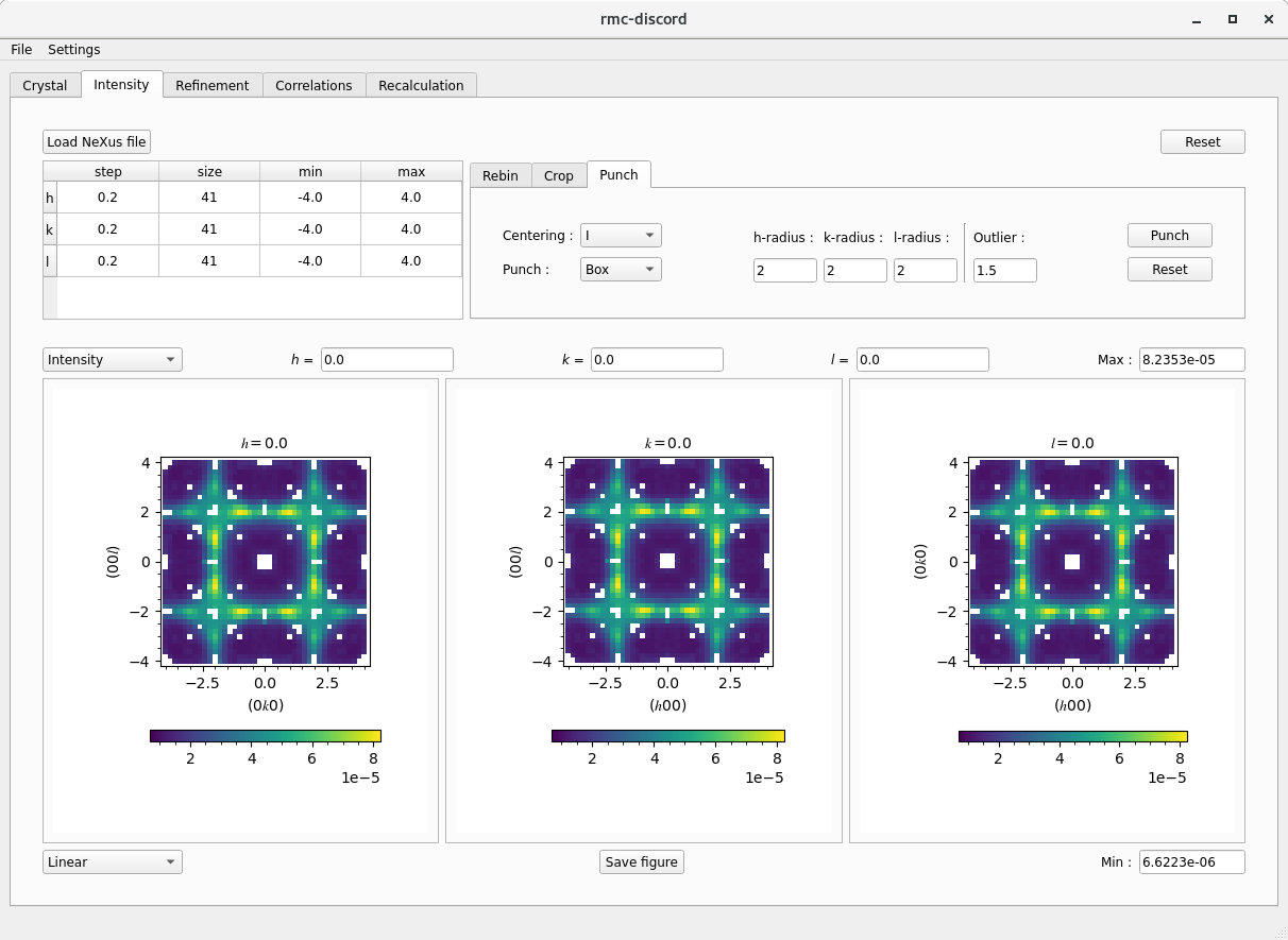
Crystal tab

Hints

• View the data in logarithmic scale to better observe the diffuse scattering.
• Select a region of interest that covers at least the primitive features of the observed diffuse scattering.
• Check for complete Bragg peak removal by switching between linear and logarithmic scaling.

Refinement tab

Setup and run a refinement.

1. Choose the refinement type by selecting the Magnetic, Occupational, or Displacive check box
   • Under each corresponding tab is a set of options relevant to that disorder type.
   • Choose Magnetic and leave the check box marked for Fixed moment
2. Set the refinement temperature prefactor and decay constant
   • The temperature Prefactor is the initial temperature.
   • Start at 1e+4.
   • The decay Constant is the rate at which the temperature decreases with each move as a Newtonian cooling function. - Start at 1e-3.
3. Choose between a single run or Batch job by specifying the number of runs
   • More runs can be averaged together to improve statistics.
4. Choose the Gaussian filter size for each \(h\), \(k\), and \(l\) size in number of pixels
   • Using Gaussian filtering reduces the noise at the expense of increasing the time of the refinement.
   • Choose 1.0x1.0x1.0 to start.
5. Start the refinement by clicking Run
   • The refinement may be stopped by clicking Stop.
   • Once stopped, the refinement may be continued or Reset for a new refinement.
   • View the intensity plot type to compare the Calculated and Experiment datasets.
   • Change the slice, scaling, and colorbar limits.
   • View different refinement static plots.

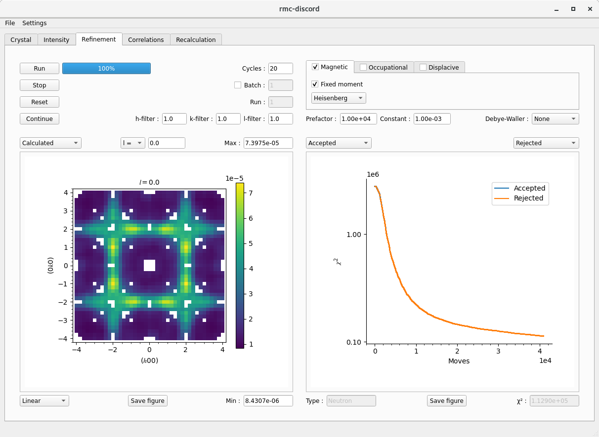
Crystal tab

Hints

• One cycle is defined as the number of moves equal to the number of atoms in the supercell.
  • Typically 100 cycles is sufficient to obtain a good refinement.
• Start off with only a few cycles (e.g. 10) to check the temperature prefactor and decay constant.
  • At the beginning, the temperature needs to be high enough such that most bad moves are accepted and very few are rejected.
  • The decay rate should be cool the system gradually such that more and more bad moves are rejected, and by the end, nearly any bad moves are accepted.
  • Cooling too quickly can quench the system into a metastable state.
  • Increasing the number of cycles by 10 typically requires decreasing the decay rate by a factor of 10 to keep a similar cooling schedule.
• Increasing the number of batch jobs improves the statistics of the correlations and the recalculated diffuse scattering pattern.

Correlations tab

After completing a refinement, the pair correlations can be calculated.

1. There are two tabs for calculating correlations: Spherical average and Three-dimensional
   • In each, the Fraction determines the largest separation vector that can be constructed multiplying this value by the longest separation vector possible in the supercell.
   • In each, the Tolerance corresponds to the maximum number of decimal places for distinguishing unique pairs.
   • Specifying 1e-2, for example, means that distances 0.333 and 0.334 are equivalent distances since they round to 0.33 using two decimal places. - The Average check box averages common separation vectors with different atom-pair types.
   • By unclicking Average, it is possible to only plot certain atom-pair types by utilizing the check boxes in the table. - The correlations may be saved as either a CSV file or VTK file which can be opened in external programs like ParaView for visualization.
2. Calculate the one-dimensional and three-dimensional correlations
   • In the upper right of each tab are the different correlation options: Magnetic, Occupancy, and Displacement
   • Select Magnetic type to and click Calculate to obtain the correlations.
   • Increase the Fraction to 0.5. - In the upper left of each tab is the option to plot the Correlations or Collinearity (if Magnetic or Displacement). - In the bottom left is the option to plot in Linear or Logarithmic scale.
3. The additional options for Three-dimensional correlations include choosing an \(hkl\) slice
   • Use integer \(h\), \(k\), and \(l\) to specify the Miller plane.
   • Choose a distance \(d\) from the origin where \((hkl)\cdot[uvw]=d\).

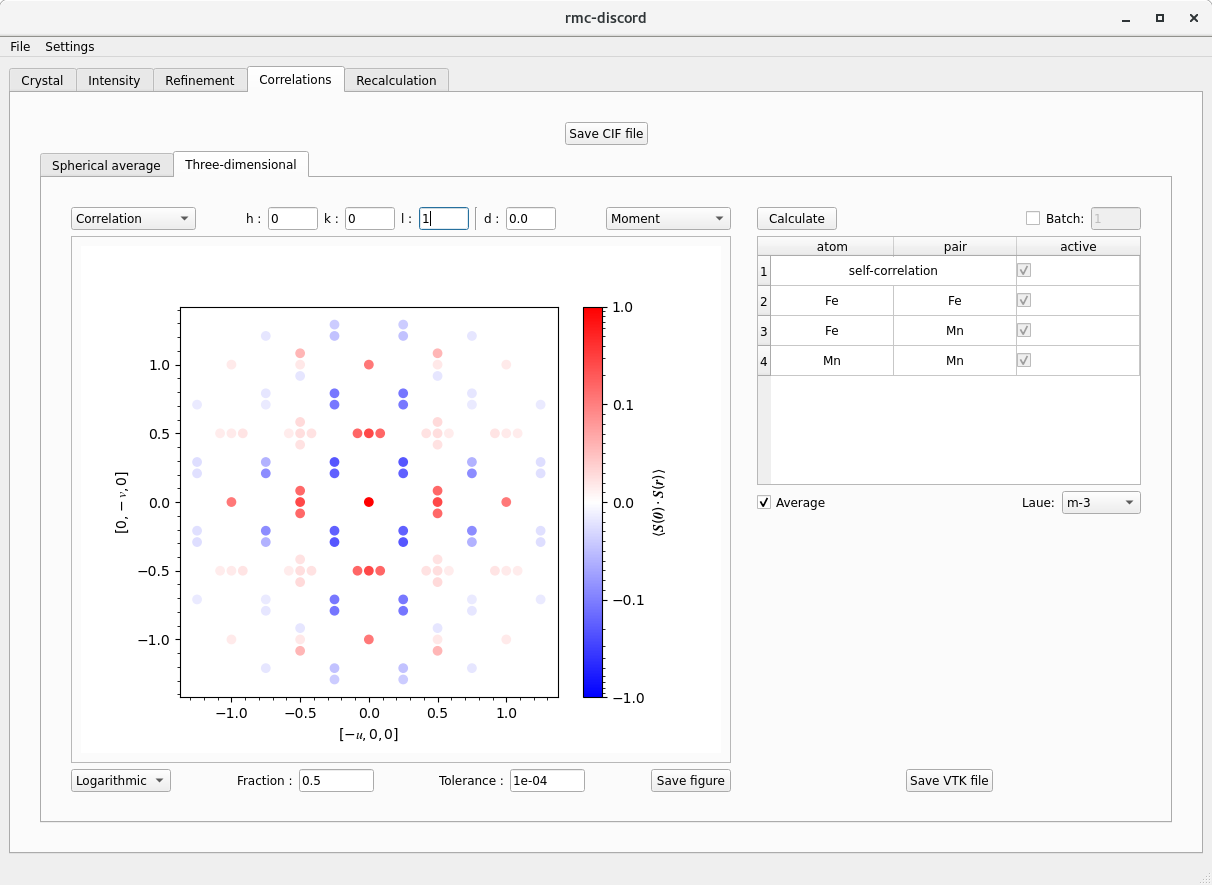
Crystal tab

Hints

• Start with a small Fraction (e.g. 0.125) and gradually increase it by small increments up to 1.0 to extend the cutoff distance of pair correlation calculation.
  • Specifying too large a fraction will take more time and consume more memory than may be available.
• Increase the Tolerance (e.g. 1e-4 to 1e-3) if more unique pairs by separation vector are identified than actually exist.
  • Unique pairs are identified by common atom pair type and separation distance(s).

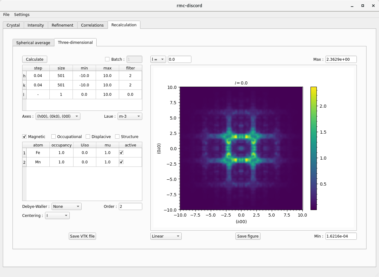
Recalculation tab

Crystal tab

Hints

• Although it is possible to recalculate the full volume of reciprocal space, it requires more time than simply calculating a slice.
  • If specifying a slice, make one of the sizes of \(h\), \(k\), and \(l\) equal to 1 and set the minimum value for the slice.
• Applying Laue symmetry to the data can improve the recalculated pattern.
  • At most, the diffuse scattering will have at most the Laue symmetry of the crystal.
  • The nature of the short range ordering can have lower symmetry than that of the average structure.